All posts by kencaldeira

Geophysical constraints on the reliability of solar and wind power in the United States

We recently published a paper that does a very simple analysis of meeting electricity demand using solar and wind generation only, in addition to some form of energy storage. We looked at the relationships between fraction of electricity demand satisfied and the amounts of wind, solar, and electricity storage capacity deployed.

M.R. Shaner, S.J. Davis, N.S. Lewis and K. Caldeira. Geophysical constraints on the reliability of solar and wind power in the United States. Energy & Environmental Science, DOI: 10.1039/C7EE03029K (2018).  (Please email for a copy if you can’t get through the paywall.)

Our main conclusion is that geophysically-forced variability in wind and solar generation means that the amount of electricity demand satisfied using wind and solar resources is fairly linear up to about 80% of annually averaged electricity demand, but that beyond this level of penetration the amount of added wind and solar generation capacity or the amount of electricity storage needed would rise sharply.

Obviously, people have addressed this problem with more complete models. Notable examples are the NREL Renewable Electricity Futures Study and another is the NOAA study (McDonald, Clack et al., 2016). These studies have concluded that it would be possible to eliminate about 80% of emissions from the U.S. electric sector using grid-inter-connected wind and solar power. In contrast, other studies (e.g., Jacobson et al, 2015) have concluded that far deeper penetration of intermittent renewables was feasible.

What is the purpose of writing a paper that uses a toy model to analyze a highly simplified system?

shaner-fig1a

Fig 1b. from Shaner et al. (E&ES, 2018) illustrating variability in wind and solar resources, averaged over the entire contiguous United States based on 36 years of weather data. Also shown is electricity demand for a single year.

The purpose of our paper is to look at fundamental constraints that geophysics places on delivery of energy from intermittent renewable sources.  For some specified amount of demand and specified amount of wind and solar capacity, the gap between energy generation and electricity demand can be calculated. This gap would need to be made up by some combination of (1) other forms of dispatchable power such as natural gas, (2) electricity storage, for example as in batteries or pumped hydro storage, or (3) reducing electricity loads or shifting them in time. This simple geophysically-based calculation makes it clear how big a gap would need to be filled.

Our simulations corresponds to the situation in which their is an ideal and perfect continental scale electricity grid, so we are assuming perfect electricity transmission. We also assume that batteries are 100% efficient. We are considering a spherical cow.

Part of the issue with the more complicated studies is that the models are black boxes, and one has to essentially trust the authors that everything is OK inside of that black box, and that all assumptions have been adequately explained. [Note that Clack et al. (2015) do describe the model and assumptions used in McDonald, Clack et al. (2016) in detail, and that the NREL study also contains substantial methodological detail.]

In contrast, because we are using a toy model, we can include the entire source code for our toy model in the Supplemental Information to our paper. And all of our input data is from publicly available sources. So you don’t have to trust us. You can look at our code and see what we did. If you don’t like our assumptions, modify the assumptions in our code and explore for yourself. (If you want the time series data that we used, please feel free to request them from me.)

Our key results are summarized in our Fig. 3:

Shaner-Fig3

Figure 3 | Changes in the amount of demand met as a function of energy storage capacity (0-32 days) and generation.

The two columns of Fig. 3 show the same data: the left column is on linear scales; the right column has a log scale on the horizontal axis. [In a wind/solar/storage-only system, meeting 99.9% of demand is equivalent to about 8.76 hours of blackout per year, and 99.99% is equivalent to about 53 minutes of blackout per year.]

The left column of Fig. 3 shows, for various mixes of wind and solar, that the fraction of electricity demand that is met by introducing intermittent renewables at first goes up linearly — if you increase the amount of solar and/or wind power by 10%, the amount of generation goes up by about 10%, and is relatively insensitive to assumptions about electricity storage.

From the right column of Fig. 3, it can be seen that that as the fraction of electricity demand satisfied by solar and/or wind exceeds about 80%, then the the amount of generation  and/or the amount of electricity storage required increases sharply. It should be noted that even in the cases in which 80% of electricity is supplied by intermittent renewables on the annual average, there are still times when wind and solar is providing very little power, and if blackouts are to be avoided, the gap-filling dispatchable electricity service must be sized nearly as large as the entire electricity system.

This ‘consider a spherical cow’ approach shows that satisfying nearly all electricity demand with wind and solar (and electricity storage) will be extremely difficult given the variability and intermittency in wind and solar resources.

On the other hand, if we could get enough energy storage (or its equivalent in load shifting) to satisfy several weeks of total U.S. electricity demand, then mixes of wind and solar might do a great job of meeting all U.S. electricity demand. [Look at the dark green lines in the three middle panels in the right column of Fig. 3.] This is more-or-less the solution that  Jacobson et al. (2015) got for the electric sector in that work.

Our study, using very simple models and a very transparent approach, is broadly consistent the findings of  the NREL, NOAA, and  Jacobson et al. (2015) studies, which were done using much more comprehensive, but less transparent, models. Our results also suggest that a main difference in conclusions between the NREL and NOAA studies and the Jacobson et al. (2015) study is that Jacobson et al. (2015) assume the availability of large amounts of energy storage, and that this is a primary factor differentiating these works. (The NOAA study showed that one could reduce emissions from the electric sector by 80% with wind and solar and without storage if sufficient back-up power was available from natural gas or some other dispatchable electricity generator.)

All of these studies share common ground. They all indicate that lots more wind and solar power could be deployed today and this would reduce greenhouse gas emissions. Controversies about how to handle the end game should not overly influence our opening moves.

There are still questions regarding whether future near-zero emission energy systems will be based on centralized dispatchable (e.g., nuclear and fossil with CCS) or distributed intermittent (e.g., wind and solar) electricity generation. Nevertheless, the climate problem is serious enough that for now we might want to consider an ‘all of the above’ strategy, and deploy as fast as we can the most economically efficient and environmentally acceptable energy generation technologies that are available today.

swatch-white_8

MZJ Hydro Explainer

If energy storage is abundant, then that storage can fill the gap between intermittent electricity generation (wind and solar) and variable electricity demand. Jacobson et al. (PNAS, 2015) filled this gap, in part, by assuming that huge amounts of hydropower would be available.

The realism of these energy storage assumption was questioned by Clack et al. (PNAS, 2017), but Clack et al. (PNAS, 2017) went further and asserted that Jacobson et al. (PNAS, 2015) contained modeling errors. A key issue centers on the capacity of hydroelectric plants. The huge amount of hydro capacity used by Jacobson et al. (PNAS, 2015) is necessary to achieve their result, yet seems inconsistent with the information provided in their tables.

Clack et al. (PNAS, 2017) in their Fig. 1, reproduced Fig. 4b from Jacobson et al. (2015), over a caption containing the following text:

F1.large

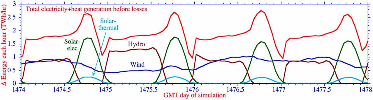
This figure (figure 4B from ref. 11) shows hydropower supply rates peaking at nearly 1,300 GW, despite the fact that the proposal calls for less than 150 GW hydropower capacity. This discrepancy indicates a major error in their analysis. 

(A dispatch of 1 TWh/hr is equivalent to dispatch at the rate of 1000 GW.)

Since the publication of Clack et al. (PNAS, 2017), Jacobson has asserted the apparent inconsistency between what is shown in Fig. 4b of Jacobson et al. (PNAS, 2015) and the numbers appearing in their text and tables was in fact intentional, and thus no error was made. Mark Z. Jacobson went so far as to claim that the statement that there was a major error in the analysis constituted an act of defamation that should be adjudicated in a court of law.

The litigious activities of Mark Z. Jacobson (hereafter, MZJ) have made people wary of openly criticizing his work.

I was sent a Powerpoint presentation looking into the claims of Jacobson et al. (PNAS, 2015) with respect to this hydropower question, but the sender was fearful of retribution should this be published with full attribution. I said I would  take the work and edit it to my liking and publish it here as a blog post, if the primary author would agree. The primary author wishes to remain anonymous.

I would like to stress here that this hydro question is not a nit-picking side-point. In the Jacobson et al. (PNAS, 2015) work, they needed the huge amount of dispatchable power represented by this dramatic expansion of hydro capacity to fill the gap between intermittent renewable electricity generation and variable electricity demand.


In the text below, Jacobson et al. (E&ES, 2015) refers to:

Jacobson MZ, et al. (2015) 100% clean and renewable wind, water, and sunlight (WWS) all-sector energy roadmaps for the 50 United States. Energy Environ Sci 8:2093–2117.

Jacobson et al (PNAS, 2015) refers to:

Jacobson MZ, Delucchi MA, Cameron MA, Frew BA (2015) Low-cost solution to the grid reliability problem with 100% penetration of intermittent wind, water, and solar for all purposes. Proc Natl Acad Sci USA 112:15060–15065.

and Clack et al (PNAS, 2017) refers to:

Clack, C.T. M, Qvist, S. A., Apt, J., Bazilian, M., Brandt, A. R., Caldeira, K., Davis, S. J., Diakov, V., Handschy, M. A., Hines, P. D. H., Jaramillo, P., Kammen, D. M., Long, J. C. S., Morgan, M. G., Reed, A., Sivaram, V., Sweeney, J., Tynan, G. R., Victor, D. G., Weyant, J. P., Whitacre, J. F. Evaluation of a proposal for reliable low-cost grid power with 100% wind, water, and solar. Proc Natl Acad Sci USA  DOI: 10.1073/pnas.1610381114.


Jacobson et al. (E&ES, 2015) serves as the primary basis of the capacity numbers in Jacobson et al. (PNAS, 2015)

May 25, 2015: Mark Z. Jacobson et al. publish paper in Energy & Environmental Science (hereafter E&ES), providing a “roadmap” for the United States to achieve 100% of energy supply from “wind, water, and sunlight (WWS).”

Picture1

To demonstrate that the roadmaps in Jacobson et al. paper (E&ES, 2015) can reliably match energy supply and demand at all times, that study cites forthcoming study (Ref. 2) that uses “grid integration model” .

Picture6Picture7

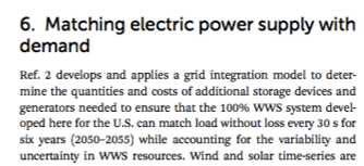
Ref. 2 is the at-that-point-forthcoming PNAS paper, “A low-cost solution to the grid reliability problem with 100% penetration of intermittent wind, water, and solar for all purposes” “in review” at PNAS.

This establishes the link between the two papers:

(1) The E&ES paper provides the “roadmap” describing the mix of renewable energy resources needed to supply the US;
(2) The PNAS paper then attempts to demonstrate the operational reliability of this mix of resources.


Jacobson et al. (E&ES, 2015) makes it clear that ‘capacity’ refers to ‘name-plate capacity’

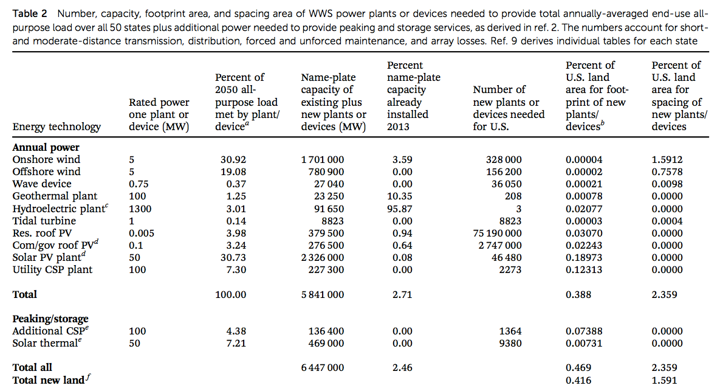
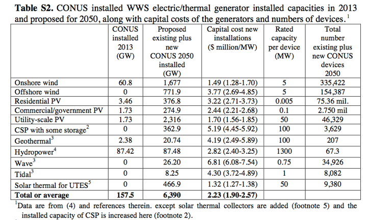
Table 2 of the E&ES paper explicitly describes the “rated power” and “name-plate capacity” of all renewable energy and energy storage devices installed in the 100% WWS roadmap for the United States. Both of these terms refer to the maximum instantaneous power that a power plant can produce at any given moment. These are not descriptions of average output, and nowhere in the table’s lengthy description does Jacobson et al. (E&ES, 2015) claim that hydroelectric power is described differently in this table than the other resources.

The table states that the total nameplate capacity or maximum rated power output of hydroelectric generators in Jacobson et al. (E&ES, 2015) is 91,650 megawatts (MW). In addition, column 5 states that 95.87% of this final installed capacity is already installed in 2013. Only 3 additional new hydroelectric plants at a size of 1,300 MW each, for a total addition of 3,900 MW over existing hydroelectric capacity are included in Jacobson et al. (E&ES, 2015) .

Picture2

Picture3


Jacobson et al. (E&ES, 2015) describes hydro capacity assumptions in some detail

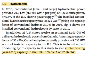
Section 5.4 of the E&ES paper provides additional textual description of the WWS roadmap’s assumptions regarding hydroelectric capacity.

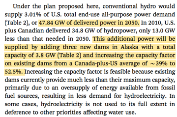
The text states that the total existing hydroelectric power capacity assumed in the WWS roadmap is 87.86 gigawatts (GW; note 1 GW = 1,000 MW).

It further states that only three new dams in Alaska with a total capacity of 3.8 GW are included in the final hydroelectric capacity in the WWS roadmap.

Note that throughout this text, Jacobson et al. (E&ES, 2015) distinguish between “delivered power,” a measure of average annual power generation, and “total capacity,” a measure of maximum instantaneous power production capability. It is this later “total capacity” figure that matches the “nameplate capacity” in Table 2 of 87.86 GW in the 100% WWS Roadmap for 2050.

The text explicitly states that the average delivered power from hydroelectric generators is 47.84 GW on average in 2050.

In Jacobson et al. (E&ES, 2015), the authors state both the maximum power production capability from hydroelectric power assumed in the WWS roadmap and distinguish this from the separately reported average delivered power from these facilities over the course of a year.

Picture4Picture5

Most of the capacity numbers appearing in Jacobson et al. (2015) come from the US Energy Administration. They define what is meant by capacity as represented by their numbers:

Generator nameplate capacity (installed):  The maximum rated output of a generator, prime mover, or other electric power production equipment under specific conditions designated by the manufacturer. Installed generator nameplate capacity is commonly expressed in megawatts (MW) and is usually indicated on a nameplate physically attached to the generator.

Generator capacity: The maximum output, commonly expressed in megawatts (MW), that generating equipment can supply to system load, adjusted for ambient conditions.

The remainder of Section 5.4. discusses several possible ways in which additional hydroelectric power capacity could be added in the United States without additional environmental impact, if it is not possible to increase the average power production from existing hydroelectric dams as Jacobson et al. (E&ES, 2015) assume is possible.

Picture8Picture9

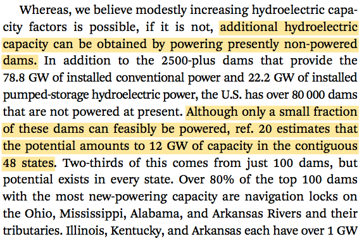
This text describes the potential to add power generation turbines to existing unpowered dams and cites a reference estimating a maximum of 12 GW of additional such capacity possible in the continguous 48 states.

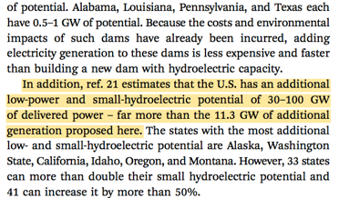
The text also describes the potential for new low-power and small hydroelectric dams, citing a reference that estimates that 30-100 GW of average delivered power—or roughly 60-200 GW of total maximum power capacity at Jacobson et al.‘s (E&ES, 2015) assumed average production of 52.5% of maximum power for each hydroelectric generator.

Nowhere in this lengthy discussion of the total hydroelectric capacity assumed in the WWS roadmap and additional possible sources of hydroelectric capacity does Jacobson et al. (E&ES, 2015) mention the possibility of adding over 1,000 GW of additional generating capacity to existing dams by adding new turbines.

The May 2015 E&ES paper by MZJ et al. explicitly states that the maximum possible instantaneous power production capacity of hydroelectric generators in the 100% WWS roadmap for the 50 U.S. states is 91.65 GW.

Jacobson et al. (E&ES, 2015) also explicitly distinguishes maximum power capacity from average delivered power in several instances. The later is reported as 47.84 GW on average in 2050 for the 50 U.S. states.

Additionally, the authors explicitly state that 3.8 GW of the total hydro capacity in the 50 state WWS roadmap comes from new dams in Alaska. This is in addition to 0.438 GW of existing hydro capacity in Alaska and Hawaii as reported in the paper’s Fig. 4. This is important to note, because Alaska and Hawaii are excluded from the simulations in Jacobson et al. (PNAS, 2015).

The E&ES companion paper to the Jacobson et al. (PNAS, 2015) therefore explicitly establishes that the maximum possible power capacity that could be included in the PNAS paper in the contiguous 48 U.S. states is 87.412 GW (e.g. 91.65 GW in the 100% WWS roadmap for the 50 US states, less 3.8 GW of new hydropower dams in Alaska and 0.438 GW of existing hydro capacity in Alaska & Hawaii).


Summary of key relevant facts about Jacobson et al. (E&ES, 2015)

In summary, the May 2015 Jacobson et al. (E&ES, 2015) paper establishes several facts:

  1. The E&ES paper explicitly states that the maximum possible instantaneous power production capacity of hydroelectric generators in the 100% WWS roadmap for the 50 U.S. states is 91.65 GW (inclusive of imported hydroelectric power from Canada).
  2. The E&ES paper also explicitly distinguishes maximum power capacity from average delivered power. The later is reported as 47.84 GW on average in 2050 for the 50 U.S. states.
  3. The E&ES paper explicitly states that 3.8 GW of the total hydropower capacity in the 50 state WWS roadmap comes from new dams in Alaska and reports that existing capacity in Alaska and Hawaii totals 0.438 GW. This is relevant, because Alaska and Hawaii are excluded from the simulations in the Jacobson et al. (PNAS, 2015) which focuses on the contiguous 48 U.S. states.
  4. The E&ES companion paper to Jacobson et al. (PNAS, 2015) therefore explicitly establishes that the maximum possible power capacity that could be included in the PNAS paper in the contiguous 48 U.S. states is no more than 87.412 GW.
  5. No where in Jacobson et al. (E&ES, 2015) do the authors discuss or contemplate adding more than 1,000 GW of generating capacity to existing hydropower facilities by adding new turbines and penstocks. In contrast, the paper explicitly discusses several other possible ways to add a much more modest capacity of no more than 200 GW of generating capacity by constructing new low-power and small hydroelectric dams.
  6. Jacobson et al. (E&ES, 2015) establishes that Jacobson et al. (PNAS, 2015) is a companion to this E&ES paper and that the purpose of the PNAS paper is to confirm that the total installed capacity of renewable energy generators and energy storage devices described in the 100% WWS roadmap contained in the E&ES paper can reliably match total energy production and total energy demand at all times. The total installed capacities for each resource, including hydroelectric generation, described in the E&ES paper, therefore form the basis for the assumed maximum generating capacities in the PNAS paper.


Jacobson et al. (PNAS, 2015) relies on hydro capacity numbers from Jacobson et al. (E&ES, 2015)

December 8, 2015: The paper “Low-cost solution to the grid reliability problem with 100% penetration of intermittent wind, water, and solar for all purposes” by Jacobson et al. (PNAS, 2015) is published in PNAS as the companion to the May 2015 Jacobson et al. (E&ES, 2015) paper.

Picture10
Picture11

Jacobson et al. (PNAS, 2015) describes existing (year-2010) hydro capacity to be 87.86 GW.
Picture4

The text further establishes that the installed capacities for each generator type for the continental United States (abbreviated “CONUS” in the text) are based on ref. 22, which is Jacobson et al. (E&ES, 2015).

Picture13

“Installed capacity” is a term of art referring to maximum possible power production, not average generation. The paper’s description of “Materials and Methods” states the the “installed capacities” of each renewable generator type are described in the Supplemental Information Table S2 of Jacobson et al. (PNAS, 2015).

Table S2 of the Supplemental Information for the PNAS paper explicitly states the “installed capacity” or maximum possible power generation of each resource type in the Continental United States used in the study.

The explanatory text for this paper again establishes that all installed capacities for all resources except solar thermal and concentrating solar power (abbreviated “CSP” in the text) are taken from Jacobson et al. (E&ES, 2015), adjusted to exclude Hawaii and Alaska. Jacobson et al. (E&ES, 2015) is ref. 4 in the Supplemental Information for Jacobson et al. (PNAS, 2015).

Picture14

Reference 4  (E&ES, 2015).

Picture15

Total installed hydroelectric capacity in Table S2 of Jacobson et al. (PNAS, 2015) is stated as 87.48 GW. This is close to the 87.412 GW of total nameplate power capacity of hydroelectric generators in the 50 U.S. states roadmap, less the new hydro dams in Alaska and existing hydropower capacity in Alaska and Hawaii.

Footnote 4 notes that hydro is limited by ‘annual power supply’ but does not mention that instantaneous generation of electricity is also limited by hydro capacity:

Picture18

Additionally, columns 5 & 6 of Table S2 separately state the “rated capacity” per device and the total number of existing and new devices in 2050 for each resource.

“Rated capacity” is a term of art referring to the maximum possible instantaneous power production for a power plant.

The rated capacity for each hydroelectric device or facility is stated as 1,300 MW and the total number of hydroelectric devices is stated as 67.3. This yields exactly 87,480 MW or 87.48 GW, the installed capacity reported for hydroelectric power in column 3. This provides further corroboration that the 87.48 GW of installed capacity reported refers to maximum rated power generation capabilities of all hydroelectric generators in the simulation, not their average generating capacity as MZJ asserts.

Nowhere in this table, its explanatory text in the Supplemental Information, or the main text of the PNAS paper do the authors establish that they assume more than 1,000 GW of additional hydroelectric generating turbines to existing hydroelectric facilities, as MZJ will later assert.

In contrast, the table establishes that the authors assume that total installed hydroelectric capacity in the Continential United States is assumed to increase from 87.42 GW in 2013 to 87.48 GW in 2050, or an increase of only 0.06 GW or 60 MW.


The hydro power capacity represented in the Jacobson et al. (PNAS, 2015) tables is inconsistent with the amount of hydro capacity used in their simulations

Despite explicitly stating that the maximum rated capacity for all hydropower generators in the PNAS paper’s WWS system for the 48 continental United States is 87.48 GW, Fig. 4 of  Jacobson et al. (PNAS, 2015) shows hydropower facilities generating more than 1,000 GW of power output sustained over several hours on the depicted days.

Picture20

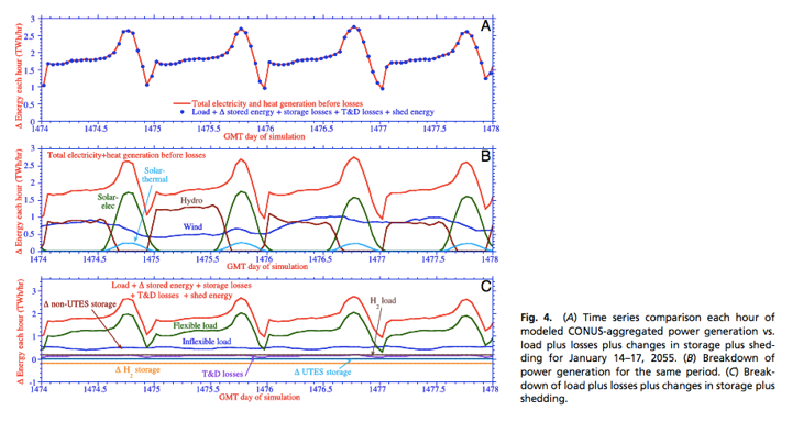
Examination of the detailed LOADMATCH simulation results (available from MZJ upon request) reveals that the maximum instantaneous power generation from hydropower facilities in the simulations performed for Jacobson et al. (PNAS, 2015) is 1,348 GW, or 1,260.5 GW more (about 15 times more) than the maximum rated capacity reported in Table S2.

It is therefore clear that the LOADMATCH model does not constrain maximum generation from hydropower facilities to the 87.48 GW of maximum rated power capacity stated in Table S2.

(Note that hydropower facilities also dispatch at 0 GW for many hours of the simulation. It therefore appears that the LOADMATCH model neither applies a maximum generation constraint of 87.48 GW or any kind of plausible minimum generation constraint for hydropower facilities.)


Summary of key facts related to hydro capacity in Jacobson et al. (PNAS, 2015)

In summary, the December 8, 2015 PNAS paper establishes the following facts:

  1. The installed capacity used in the simulations in Jacobson et al. (PNAS, 2015) is reported in Table S2 of the Supplemental Information for that paper. The total installed hydroelectric capacity or maximum possible power generation reported in Table S2 is stated as 87.48 GW.
  2. This maximum capacity figure is also separately corroborated by taking the rated power generating capacity per device and total number of devices reported in Table S2, which also yields a maximum rated power production from all hydroelectric generators of 87.48 GW.
  3. Table S2 states the the authors only assume 0.06 GW of additional hydroelectric power capacity is added between 2013 and 2050.
  4. Nowhere in the text of Jacobson et al. (PNAS, 2015), its Supplemental Information document, or the explanatory text for Table S2 do the authors state that the term “installed capacity” or “rated capacity per device” for each resource reported in the table is used in any other way than the standard terms of art indicating maximum power generation capability. Nor do the authors establish that total installed capacity of hydroelectric generation is described differently in this table than the other resources and refers instead to average annual delivered power as MZJ claims.
  5. Jacobson et al. (PNAS, 2015) also references and uses Jacobson et al. (E&ES, 2015) to establish the installed power generating capacity of each resource in the simulations performed in the PNAS paper, with the explicit exception of solar thermal and concentrating solar power. The maximum rated power from hydroelectric generation reported in Table S2 of 87.48 GW is consistent (within 68 MW) with the 87.412 GW of name-plate generating capacity reported in the E&ES paper for the 50 U.S. states less three new hydropower dams in Alaska and existing hydro capacity in Alaska and Hawaii reported in the E&ES paper.Recall also that the average delivered power from hydroelectric generators was explicitly and separately stated in the E&ES paper as 47.84 GW for the 50 U.S. states, and is therefore no more than 47 GW for the 48 Continential US states. The reported “installed capacities” for hydroelectric generation in PNAS Table S2 is therefore entirely consistent with the “name-plate capacity” reported in the E&ES paper and is not consistent with the average delivered power from hydroelectric generation reported in the E&ES paper.
  6. Despite establishing a maximum rated power capacity of 87.48 GW, the simulations performed for Jacobson et al. (PNAS, 2015) dispatch hydropower at as much as 1,348 GW, or 1,260.5 GW more than the maximum rated capacity reported in Table S2.


Conclusions

Given available information in the published papers, a reasonable reader should interpret the “installed capacity” or “rated capacity” figures explicitly reported in Table S2 of the Jacobson et al. (2015) paper as referring to maximum generating capacity, because that is the definition used by the studies reported on in the table.

This assertion that the 1,348 GW of maximum hydro generation used in the LOADMATCH simulations for the PNAS paper constitutes an intentional but entirely unstated assumption rather than a modeling error (e.g. a failure to impose a suitable capacity constraint on maximum hydro generation in each time period) is, as we understand it, the primary basis for MZJ’s lawsuit alleging that Christopher Clack and the National Academies of Sciences (publishers of PNAS) intentionally misrepresented his work and thus defamed his person.

A reading of the E&ES and PNAS papers establishes that the MZJ et al. did not omit explicit description of the total rated power capacity of hydroelectric facilities. In point of fact, the authors establish in multiple ways that the maximum power capacity for hydroelectric facilities in the PNAS WWS study for the 48 continental United States is 87.48 GW, not the 1,348 GW actually dispatched by the LOADMATCH model.

Thus, information in the E&ES and PNAS papers do not appear to be consistent with MZJ’s assertions that he and his coauthors had intentionally meant to add more than 1,000 GW of generating capacity to existing hydropower facilities in their model.  (It is outside the scope of this analysis to discuss the plausibility of adding more than 1,000 GW of hydro capacity to existing dams.) Nor does the available evidence indicate that they intentionally assumed more than 1,000 GW of additional hydro capacity and then simply failed to disclose this assumption at any point in either of the two papers.  Such failure to explicitly describe such a large and substantively important assumption to readers and peer reviewers might itself constitute a breach of academic standards.

The operation of the LOADMATCH model is inconsistent with the maximum power generating capacity of hydropower facilities explicitly stated in Jacobson et al. (PNAS, 2015) and in the companion paper, Jacobson et al. (E&ES, 2015) upon which the generating capacities are based. Whether you call failure to impose a suitable capacity constraint on maximum hydro generation in each time period a “modeling error” is up to you, but that would seem to be an entirely reasonable interpretation based on the available facts.

swatch-white_8

Ocean heat flux and open ocean wind energy

I posted this on our professional web site (http://carnegieenergyinnovation.org), but thought it useful to repost here.

Anna Possner  and I recently published a study in the Proceedings of the National Academy of Sciences, titled “Geophysical potential for wind energy over the open oceans“.

It is well known that there is enough wind energy to power civilization,  and that wind speeds tend to be higher over the open oceans.  What wasn’t known was whether winds over the oceans tend to be stronger because the ocean presents a smooth surface without any mountains, trees, or houses to slow the flow, or whether there really is something special about the oceans that promotes stronger winds.

Anna performed a set of numerical climate model simulations to evaluate the maximum rate at which the atmosphere could transport kinetic energy (wind energy) downward to the surface, and how that varied from place to place and from season to season.

We noticed that there was a very strong correlation between the rate at which energy could be extracted near the surface (which becomes limited by the rate at which the atmosphere can transport energy downward) and the amount of heat  streaming out of the ocean into the atmosphere. The following figure embellishes Figure S10 from the Supporting Material for the paper mentioned above.

The land surface can store heat in the summer and release it in the winter but cannot transport heat from one place to another. In contrast, ocean currents can transport heat from low latitude to high latitude regions. Ocean heat transport can generate surface temperature contrasts (between land and sea and between different ocean areas). These temperature contrasts can contribute to unsettled and stormy activity in the atmosphere that can bring wind energy downward from the middle of the atmosphere towards the surface. Buoyancy forces may also play a role, with heat of the lower atmosphere inducing some rising motion that is compensated for by downward moving air with higher amounts of kinetic energy.

The specific mechanisms are yet to be worked out in detail, but the figure above shows a relatively tight and unexpected correlation between ocean-to-atmosphere heat fluxes and the maximum sustainable wind-energy extraction rates in those locations.

Anders Levermann  asked me about global warming. Global warming induces a heat flux from the atmosphere to the ocean and so tends to reduce net ocean-to-atmosphere heat fluxes. Furthermore, heating of the ocean surface and increased high-latitude precipitation tend to increase the vertical stability of the upper ocean, inhibiting vertical mixing, and thus reducing atmosphere-ocean heat exchange. These changes are likely to be small relative to the magnitudes present in the background state, but would indicate that while today there is a huge wind energy resource in some open ocean environments, it could be a little smaller in a global warming scenario.

The scientific novelty of our study is in showing that the ocean really is different from the land when it comes to wind power potential, and that difference is largely due to the fact that the ocean can transport heat but the land cannot.  There were several good press accounts of our work, and these press accounts emphasized the resource size. We appreciate the coverage we got and understand that science journalists need to focus on what will be most interesting to a broad audience and not necessarily on the contribution that will be most interesting to our scientific colleagues.

Some of the best journalistic accounts of our work can be found in these links (sorry if you are a journalist who did a great job but I didn’t see it or forgot to link to you here):

Chris Mooney, Washington Post
Bob Berwyn, InsideClimateNews
Eli Kintisch, Science

Saying “there is enough wind energy over the open oceans to power civilization” is a little like saying “there is enough solar energy over the Sahara desert to power civilization.” It is true but of little practical value if there are other ways to provide that energy that are much cheaper and easier, and perhaps with less adverse environmental consequence. Nevertheless, I think our study gives a green light to those developing floating wind farm technologies and suggests that they can focus on low-cost resolution of engineering challenges — and that they don’t need to worry about running out of resource.

swatch-white_8

Imagine it is year 2100 and the world is a good place to be.

To create something, we must visualize it first.

Every human artifact exists first in our minds and then only later in reality.

If we want a world where nearly everyone can experience a deep sense of well-being, and where nature can flourish, we need to visualize that world and attempt to create it.

Many people have been thinking about transition paths to better futures, and often these discussions get hung up in the difficulty of getting anything done in a political environment that is oriented to short-sighted self-service of the privileged few.

Much of the climate conversation seems to hover around doom and gloom, generating feelings of frustration and despair. This negative messaging is not getting us to where we want to be.

Another approach is to attempt to visualize a range of futures that we would like to live in (or like to see the world living in) and then try to understand which of these possible futures has a feasible path leading to it from where we are now.

What would have to become true in order to make each of those futures possible? How likely is it that each of those things would become true? If we construct many such lists for many such futures, we can ask what are the items that show up again-and-again on nearly every list, and therefore is a likely requirement for making good futures be feasible futures.

This idea of trying to visualize outcomes that we want and then figure out transition paths to those outcomes has become a major organizing theme for much of the work in my group. (See http://CarnegieEnergyInnovation.orghttp://CarnegieEnergyInnovation.org)

I recently tweeted “Imagine it is year 2100 and the poorest parts of the world are prosperous and carbon free. What had to be true to make that happen?” I was surprised by the amount of conversation that this tweet generated. It suggests people are ready for some positive messaging around the climate issue.

But positive messaging must be realistic. While it is important to visualize positive futures, we should not delude ourselves into thinking that those positive futures will be easy to create.

Clipboard01

swatch-white_8

Larsen C and solar geoengineering

cxaovzcwqaa0nllPhoto: nasa.gov

Michael Thompson, of the Forum for Climate Engineering Assessment wrote me asking me about my thinking regarding the Larsen Ice Shelf and solar geoengineering. My responses, alongside others, were published on this web page:  http://ceassessment.org/larsen-c-climate-engineering-and-polar-ice-melt .

My comments are repeated here:

Ken Caldeira: “Melting in Antarctica is strongly influenced by interactions involving the circulation of seawater, and its interaction with glacial ice, sea ice, surface winds and temperature, sunlight and so on. Many important interactions are occurring on small spatial scales that have not yet been successfully integrated into models simulating large-scale phenomena — and so the influence of various possible solar geoengineering deployments on Antarctic ice sheet dynamics remains largely unknown and unexplored.

The governing hypothesis is that if warming temperatures lead to ice melt, cooler temperatures are likely to help slow or even stop that melt.

It might turn out that it is effectively impossible to cool the water adjacent to ice shelves with solar geoengineering techniques. However, I would be surprised if that turns out to be the case. My expectation is that the primary factors limiting the amount cooling produced by solar geoengineering would be unintended consequences and sociopolitical acceptance.

We should be researching the potential effectiveness and unintended consequences of using solar geoengineering techniques to reduce the amount of damage caused by climate change. However, I would want to know a lot more about potential efficacy and unintended consequences, and understand how the solar geoengineering deployment fits into the broader spectrum of efforts undertaken to avoid climate damage, before I would want to consider using solar geoengineering approaches to protect Antarctica.”

swatch-white_8


Red team, blue team

Justin Gillis of the New York Times asked me to comment on a proposal by EPA head Scott Pruitt regarding a red-team/blue-team approach to climate science. I wrote this set of possible quotes, and one of them appeared in this article: EPA to Give Dissenters a Voice on Climate, No Matter the Consensus, by Brad Plumer and Coral Davenport.


I would love to hear Scott Pruitt explain how he thinks the scientific process works. What does he think scientists are doing all day? Scientists are already spending most of their time trying to poke holes in what other scientists are saying.

The whole red team / blue team concept misunderstands what science is all about. Scott Pruitt seems to imagine that science today is like a football game with a single team on the field. In fact, science is like having thousands of people out on the field, each playing for themselves, fighting tooth and nail to show that they are right and everyone else is wrong.

We don’t want red team / blue team because science doesn’t line up monolithically for or against specific positions. Science is an ongoing process of thousands of people constantly chipping away at or refining a set of hypotheses.

Scientists in the United States have organized themselves to create the best scientific infrastructure in the world, and now we need a politician to tell scientists how to do science? If Scott Pruitt really wants to improve climate science, he should be fighting for bigger budgets for climate scientists.

Why do politicians who have never engaged in any scientific inquiry in their lives believe themselves to be the experts who should tell scientists how to conduct their business? A little more humility would be appreciated. This is yet another example of politicians engaging in unhelpful meddling in things they know nothing about.

Why is Scott Pruitt trying to ‘fix’ climate science. It is not broken. If Scott Pruitt really wanted to help climate science, he would be fighting to increase budgets for climate science research.

All of science is about one person claiming to have evidence supporting a hypothesis, and then other people trying to show that the first person was either wrong or missing something important.

Science is a constant process of scientists challenging the claims of other scientists.

Some more thoughts (written after the original email to the Times):

Isn’t science all red team? Isn’t all of science aimed at falsifying hypotheses? Popper would say that if you are trying to prove that something is true, then you aren’t doing science.

I just don’t understand which hypotheses Scott Pruitt thinks climate scientists are being insufficiently rigorous about testing. Scott Pruitt should clearly state the hypotheses that he thinks climate scientists are accepting prematurely. 

Will Pruitt commit to vigorous and effective action on emissions reduction if the main findings of climate science are shown to be sound? [Hasn’t the science already been shown to be sound?] Is the Trump Administration committed to basing policy on the best-available scientific information?

unnamed (1)

Trump, climate, and energy

The journalist Jeff Goodell asked me for some comments about Trump and his decision to not honor climate pledges made by the United States. In lightly edited form, this is what I replied, largely as stream-of-consciousness writing:

The United Nations Framework Convention on Climate Change (UNFCCC) was adopted on 9 May 1992, just over 25 years ago. The Convention was signed by then-President George H. W. Bush. The UN Framework Convention was negotiated by a Republican Administration.

In signing the Convention, President Bush spoke of “crucial long-term international efforts to address climate change”, and said “I am confident the United States will continue to lead the world in taking economically sensible actions to reduce the threat of climate change.”

Nearly 20 years ago, Marty Hoffert and I, with other colleagues, published the first peer-reviewed study outlining how much carbon-emission-free energy we would need to support economic growth while protecting our environment. So far, the world has done about one-tenth of what we projected would need to be done by now.

Hoffert_Caldeira3-1
Fig. 1. Hoffert et al., (1998) estimated that by now, nearly half of our primary power would need to come from sources that do not dump carbon dioxide pollution into the atmosphere. Even with the most generous accounting, less than 20% of our energy comes from such sources today.

I am confident that history will come to look upon the Trump Administration and his congressional co-conspirators as dark stain on American history, as a failed effort by regressive forces to return to a world that never was.

Trump and his Republican co-conspirators will be swept aside by demographic trends.

I have to believe that what is good in America will reassert itself. Compassion, tolerance, respect, and caring for others will supplant greed and fear-mongering.

With this resurgence of positive spirit, expressed through our newly restored political institutions, we will reach a national consensus that nothing can really be good for America if it is not also good for the rest of the world.

The United States will lead an energy system transition, and build a new economy with new jobs, and create an energy system that can promote economic growth while protecting natural assets.

After the Dark Ages, came the Renaissance.

We are in our political Dark Ages, but there will be a political Renaissance.

The ascent of Trump and his cohort, with all their foolish actions, are but a temporary setback. They cannot for long hold back the forces of history.

The global historical trends show people lifted out poverty, with better education, better health care, becoming more tolerant, and taking better care of the environment. These trends will continue.

Yes, there are setbacks, driven by fact-denying forces both at home and abroad, but these setbacks do not undermine broader historical trends.

The political survival of the Republicans and Democrats alike will depend on embracing these trends.

It is important that thinking, caring Americans make it clear that Trump is an aberration; he is the noise and not the signal. Our system will self correct. America will be great again.

The Democrats share responsibility for Trump and his misguided policies. They have not fought for policies that help the average person whose job is threatened by automation or globalization. They too have failed to put in place policies that recognize the magnitude of the energy system transformation that lies before us.

If two good things can come out of the Trump Administration, they will be (1) undermining the Republican Party by exposing them as craven, venal and unprincipled, and (2) re-invigorating the Democratic Party to fight for policies that are as ambitious as the problems that face us are large; these problems include health care, education, employment, and the challenge of radically transforming our energy system.

The reckless and ignorant actions undertaken by the Trump Administration are but a temporary setback. It is important to keep in mind that addressing the climate problem will involve a century-scale energy system transition, and that we have already let the clock run for a quarter-century without getting very far from the starting gate.

The United States, along with the rest of the world, will be building an energy system that does not rely on using the sky as a waste dump for our CO2 pollution.

For now, the rest of the world (and the states and non-government actors) will have to make progress without support from the White House. The next Presidential Administration will have to work harder to make up the ground we are losing now.

swatch-white_8

Learning curves and clean-energy R&D: Follow the curve or try to leap?

For most energy technologies, cost decreases with as the cumulative amount of deployment increases. Often, the cost is seen to decrease approximately the same amount with each doubling of the amount deployed. Straight line curve fits to cost data are commonly known as ‘learning curves’ and look like this:

1-s2.0-S0301421517303130-gr1Fig. 1. (from Shayegh et al., 2017) Learning curves for clean and conventional energy technologies. The horizontal axis represents cumulative quantity of electricity generation and the vertical axis represents the unit cost of electricity generation. Both scales are logarithmic. Learning rates (R) are shown in parentheses. Q0 indicates starting quantity and C0 is starting cost. With this axis scaling, straight lines represent power laws (Eq. (1)). We use data from this figure for subsequent analysis of the impact of different types of R&D (EIA, 2015, Wene, 2000 ; Rubin et al., 2015).

The idea is that as more of a technology gets deployed, people learn how to make the technology more cheaply, although economies of scale and other factors also play roles in bringing down costs.

I had the good fortune to be in a discussion with venture capitalists who were investing in companies doing research and development (R&D) on energy technologies. They mentioned that they didn’t want their R&D investment to just push them down the learning curve — they didn’t want to just learn things that they would have learned as production scaled up.

They said they want to shift the learning curve downward. They wanted to invest in innovations that would decrease cost as a result of innovations that would not come about simply by scaling up manufacture. (For example, maybe by shifting solar photovoltaic cells to a new kind of substrate.) This raises the question: If an R&D investment could reduce cost by the same amount by shifting the cost-starting-point of the learning curve downward (“curve-shifting R&D”) instead of effectively following the learning curve to that cost (“curve-following R&D”), which one would be better and how much better would it be?


To address this question, I got the help of Soheil Shayegh, a specialist in optimization and other mathematical and technical arts, and talked him into leading this project.

The “learning subsidy” is the total amount subsidy that would be needed to make a new more-expensive technology competitive with an incumbent technology. The needed subsidy to make a more expensive technology competitive in the marketplace starts out high but decreases as learning brings down the costs of the new technology (Fig 2a).

Figure 1 above shows cumulative quantity on the horizontal axis on a logarithmic scale, but such a figure can be redrawn with a linear axis, which turns the straight lines into curves. Figure 2 shows such curves for an idealized case:

1-s2.0-S0301421517303130-gr2

Fig. 2. (from Shayegh et al., 2017) Illustration of two stylized types of R&D for solar PV, a clean energy technology. (a) Learning-by-doing reduces the cost of the clean energy technology as the cumulative quantity of electricity generation increases. (b) Curve-following R&D reduces cost by producing the same knowledge as learning-by-doing, with an effect equivalent to increased cumulative quantity. (c) Curve-shifting R&D reduces cost by producing knowledge that would not have been gained by learning-by-doing, scaling the learning curve downward by a fixed percentage. The learning investment is the total subsidy necessary to reach cost parity with fossil fuels. For the same initial reduction in cost, curve-shifting R&D reduces the learning investment more than curve-following R&D. Note that horizontal and vertical scales are linear. The learning curves would be straight lines if both scales were logarithmic as in Fig. 1.

We found was that cost reductions brought about by breakthrough curve-shifting innovations were much more effective and bringing technologies closer to market competitiveness than were the same cost reductions brought about by incremental curve-following innovations. For example, that cost reductions in wind and bioenergy that come from curve-shifting research are more than 10 times more valuable than cost reductions that come about from curve-following research.

Further, we found in this idealized framework that the relative benefit of breakthrough innovations depended on only two things: (1) the initial cost of the new technology relative to the incumbent technology, and (2) the slope of the learning curve. The more expensive the new technology and the shallower the learning curve, the higher the value of breakthrough curve-shifting R&D.


I am principally a physical scientist, and Soheil Shayagh is principally some sort of mathematically-oriented engineer. To make a successful study, we needed to make some contact with the real world, or at least the academic literature on learning and technological innovation. To this end, we brought Dan Sanchez into the project. Dan thinks a lot about how public policy can help promote innovation and the deployment of new, cleaner energy technologies.

The result of our work was a study titled “Evaluating relative benefits of different types of R&D for clean energy technologies“, published in the journal Energy Policy. (Unfortunately, due to an oversight, our study ended up behind a paywall but you can email me at [email protected] to request a copy.)

Our results indicate that, even if steady curve-following research produces results more reliably, when successful, step-wise curve-shifting research produces much greater benefits.

Our simple calculations are highly idealized and schematic and are designed only to illustrate basic principles.

I infer from our study that, other things equal (and other things are never equal), government funded R&D should focus on trying to achieve step-wise curve-shifting breakthroughs.

I suppose my group’s research should also focus on trying to achieve step-wise breakthroughs, but that’s a tough challenge.


swatch-white_8

Will using a carbon tax for revenue generation create an incentive to continue CO2 emissions?

Most economists think a tax on carbon dioxide emissions is the simplest and most efficient way to get us to stop using the sky for disposal of our waste CO2. This tax could be applied when fossil fuels are extracted from the ground or imported, and credits could be given if someone could show that they permanently buried the waste CO2 underground.

This carbon tax would make fossil fuels more expensive. If the tax level continued to increase, eventually using fossil fuels (without underground CO2 disposal) would become more expensive than every other energy technology, and economics would squeeze carbon dioxide emissions our of our economy.

A tax is an anathema to most politicians. One proposal to make such a tax more palatable would be to distribute the revenue evenly on a per capita basis. Due to inequalities in income distribution, this would result in most people receiving a direct net economic benefit. This could make it politically popular. In terms of net transfer, money would be transferred from the rich and given to the poor and middle classes. Thus, a revenue-neutral carbon tax would both help eliminate carbon dioxide emissions and help reduce economic inequality. Sounds like a good thing. (Why aren’t we doing it?)

Another idea would be to institute a carbon tax to generate tax revenue that could then be used to help provide essential services such as health care, education, income subsidies, and so on. Some of the carbon tax could potentially be used to help pay down the national debt, which in the United States now stands at $165,000 per taxpayer.

Today, we have a carbon tax rate of zero and get no carbon tax revenue. When the carbon tax rate is so high that there are no longer any carbon emissions from our energy system, the carbon tax revenue will again be zero. There is some tax level in-between that would maximize revenue generation from the carbon tax. An increase in tax rate beyond this level would reduce carbon dioxide emissions so much that carbon tax revenues would start to diminish.

Whether the proceeds of the tax are distributed on a per capita basis, or used to provide essential services, people will not be happy to see tax rates rise while direct and immediate benefits from the tax decrease. These tax increases could be a tough sell for politicians. Politicians could be motivated to avoid raising the carbon tax rate, so that they can continue providing the benefits of the revenue generation to their constituents. This would result in continued CO2 emissions.


This issue had been nagging me for over a decade, and I have long tried to interest someone in taking the lead on addressing this question. (Avoiding work is one of my key objectives, so my usual strategy is to try to talk people into doing the work that I am trying to avoid doing myself.) Luckily, I was able to talk Rong Wang into addressing this problem. Because Rong is a physical scientist and not an economist, we were fortunate to be able to lure the economist Juan Moreno-Cruz into helping us.

Together, we produced a study titled “Will the use of a carbon tax for revenue generation produce an incentive to continue carbon emissions?“, and published it in Environmental Research Letters, where it is available for free download.

The key conclusion is represented in this figure:

Wang_fig 1b_170523

Figure 1b. Projected emissions under a set of standard assumptions for three scenarios: Zero carbon tax, welfare-maximizing carbon tax, and revenue-maximizing carbon tax. Under the revenue maximizing assumption, CO2 emissions continue long into the future but at a level that is lower than would occur if there were no carbon tax at all.

Our main conclusions are: For the next decades, the incentive to generate revenue would provide motivation to increase carbon tax rates and thus achieve even lower emissions than would occur at an economically optimal ‘welfare-maximizing’ tax rate. However, by the end of this century, the incentive to generate revenue could result in too low a tax rate — a tax rate that would allow CO2 emissions to persist far into the future.

Overall, I see our result as rather encouraging. Right now, the problem is that we don’t have enough disincentives on carbon emission and politicians are having trouble motivating themselves to provide this disincentive. If revenue generation provides an additional incentive (beyond the incentive of generating climate benefits) to institute a carbon tax, that is all well and good. As mentioned above, these revenues could be distributed on a per capita basis to help combat inequality, or they could be used to provide essential services.

By the end of the century, the incentive to generate revenue could become a perverse incentive to keep carbon taxes low so that CO2 emissions might continue. However, for now, the incentive to generate revenue would motivate increased carbon tax rates, which would cause carbon emissions to decrease.

Given that today’s carbon tax rate is zero, which is clearly too low, the incentive to generate revenue can help motivate politicians to do the right thing for the climate system. That is a good thing.

swatch-white_8

Climate of Risk and Uncertainty

ClimateFeedback.org contacted me asking what I thought about Bret Stephens’ first column in the New York Times. Here, is a slightly edited version of my response.

Bret Stephens’ opinion piece, titled “Climate of Complete Certainty”, is attacking a straw man. No working scientist claims 100% certainty about anything.

Science is the process of falsification. Hypotheses that have withstood a large number of attempts at falsification, and that are consistent with a large body of established theory that has also resisted falsification, are widely regarded as true (e.g., the Earth is approximately spherical). Many hypotheses of modern climate science fall into this category.

It is also true that some ‘environmentalists’ go far beyond the science in making claims, but that is not cause to denigrate the science.

Bret Stephens writes of ‘sophisticated but fallible models’ as if ‘sophisticated but fallible’ gives one license to ignore their predictions. A wide array of models of different types and levels of complexity predict substantial warming to be a consequence of continued dependence on using the sky as a waste dump for our CO2 pollution. It doesn’t take much scientific knowledge to understand that the end consequence of this process involves approximately 200 feet of sea-level rise. We already see the coral reefs disappearinga predicted consequence of our CO2 emissions. How much more do we need to lose before recognizing that our ‘sophisticated but fallible models’ are the best basis for policy that we have?

Yes, we should take uncertainty into account when developing policy, but we should recognize that those ‘sophisticated but fallible models’ are as likely to underpredict as overpredict the potential consequences of our greenhouse gas emissions.

Stephens would have been on more solid ground if he would have confined his comments to uncertainty in the ability of human systems to adapt to the relatively more certain projections of changes in the physical climate system. Will we be able to give up low-lying countries and the major coastal cities of the world (New York, London, Tokyo) without much of a transition cost? Will people in India and the Sahel be able to migrate or air-condition their way out of the harsh conditions projected for those areas? These are open questions about which well-informed people can disagree.

It is dangerous to act as if uncertainty in climate model projects justifies inaction. Uncertainty equals risk. One way to reduce uncertainty is to increase the amount and quality of climate science being conducted. Another and more important way of reducing uncertainty is to reduce human influence on the climate system. This requires a major transformation of our energy system to one that does not rely on the atmosphere as a waste dump for our CO2 pollution.

Climate science does not offer complete certainty about the future. Instead, it points to substantial risks and ways to avoid that risk.

Straw-man attacks on climate scientists do not productively advance the discussion.

For reference: My first reaction to the announcement of the The New York Times decision to hire Bret Stephens.

Clipboard01
swatch-white_8